Lec 21 part2 & 22 · CUDA 예제·warp divergence 와 domain-specific accelerator(DNN·systolic array·TPU)
정밀 정리 · 검증 2026-09-25 00:54
1개요
1.1L21 후반: CUDA vector_add 의 thread 인덱싱과 host 초기화(cudaMalloc·cudaMemcpy), control divergence 와 dynamic warp formation.
1.2L22: domain-specific accelerator 동기(performance/cost, latency, 연산 수요)와 ASIC vs FPGA trade-off.
1.3DNN 기초: perceptron·MLP·CNN·RNN 모두 matrix multiply(MAC) 중심, convolution 도 matrix multiply 로 변환.
1.4systolic array 개념·장단점·2×2 matrix multiply 예제, DSA 설계 지침, Google TPUv1 의 구조·floorplan·ISA.
2섹션별 정리 상황·문제 → 원인 → 해결
2.10:29–7:36CUDA 예제: vector_add kernel 과 thread 인덱싱
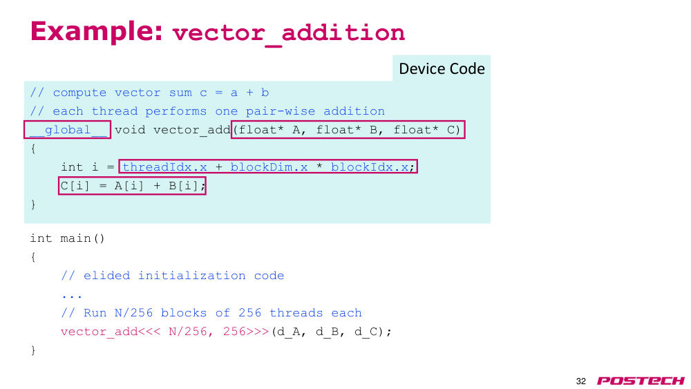
상황·문제지난 시간 이어서 CUDA 코드 예제. main 은 CPU, vector_add kernel 은 GPU 에서 실행.
원인kernel 은 N/256 개 thread block × block 당 256 thread 의 1D grid 로 launch. 각 thread 가 자기 원소를 찾아야 함.
해결i = threadIdx.x + blockDim.x * blockIdx.x 로 전역 index 계산, C[i] = A[i] + B[i]. N=1024 이면 1024 thread 가 원소 하나씩.
- __global__ = GPU 에서 실행되고 CPU 가 호출하는 함수
- N=1024 → 4 block × 256 thread. blockIdx.x=2, threadIdx.x=10 이면 256×2+10
- 2D·3D 데이터는 2D·3D grid/block 으로 확장 가능
2.1.r.1Wikipedia: Thread block (CUDA programming) ↗ · i = blockIdx.x*blockDim.x + threadIdx.x 인덱싱, warp=32 thread
2.27:39–10:52host 초기화 코드: cudaMalloc 과 cudaMemcpy
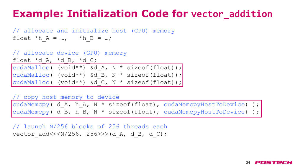
상황·문제앞 슬라이드에서 생략된 host 초기화 부분 설명.
원인CPU memory 와 GPU memory 가 분리돼 있어 두 벌 할당이 필요.
해결h_A·h_B 는 host(디스크에서 적재), d_A·d_B·d_C 는 cudaMalloc, cudaMemcpy(…HostToDevice) 로 복사 후 kernel launch. 결과는 다시 CPU 로 복사해 사용.
- cudaMalloc 으로 GPU memory 할당
- cudaMemcpyHostToDevice 로 A·B 전송
- 결과 C 의 역복사는 슬라이드에 없고 말로만 언급
2.310:56–15:47control divergence(제어 분기) 문제
상황·문제vector add 처럼 규칙적이면 GPU 를 꽉 채우지만, 불규칙한 program 은 utilization 이 낮아짐.
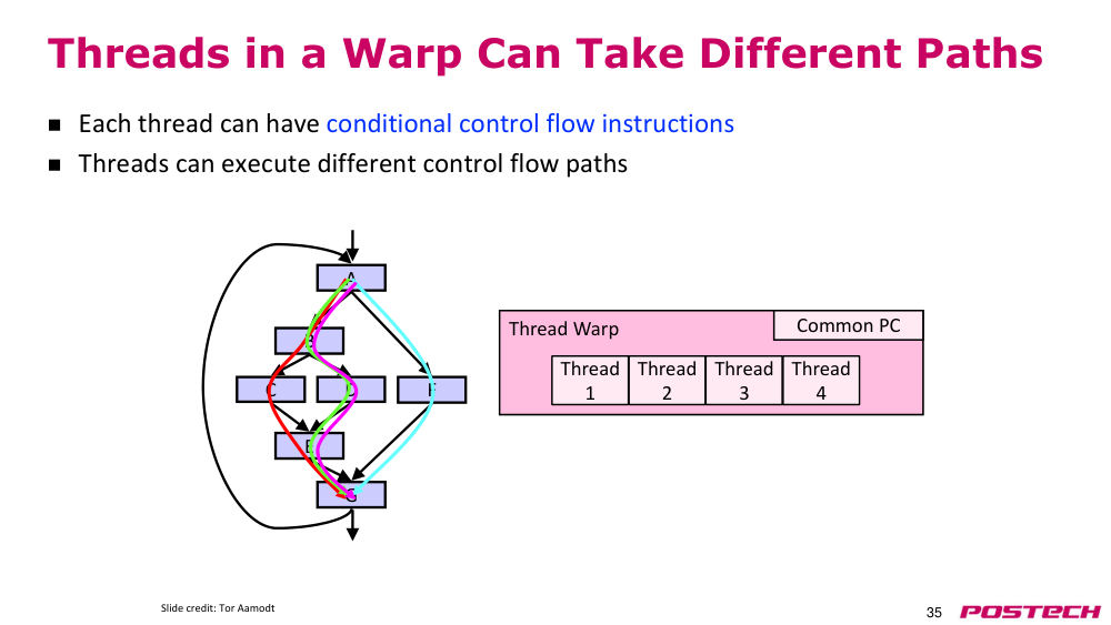
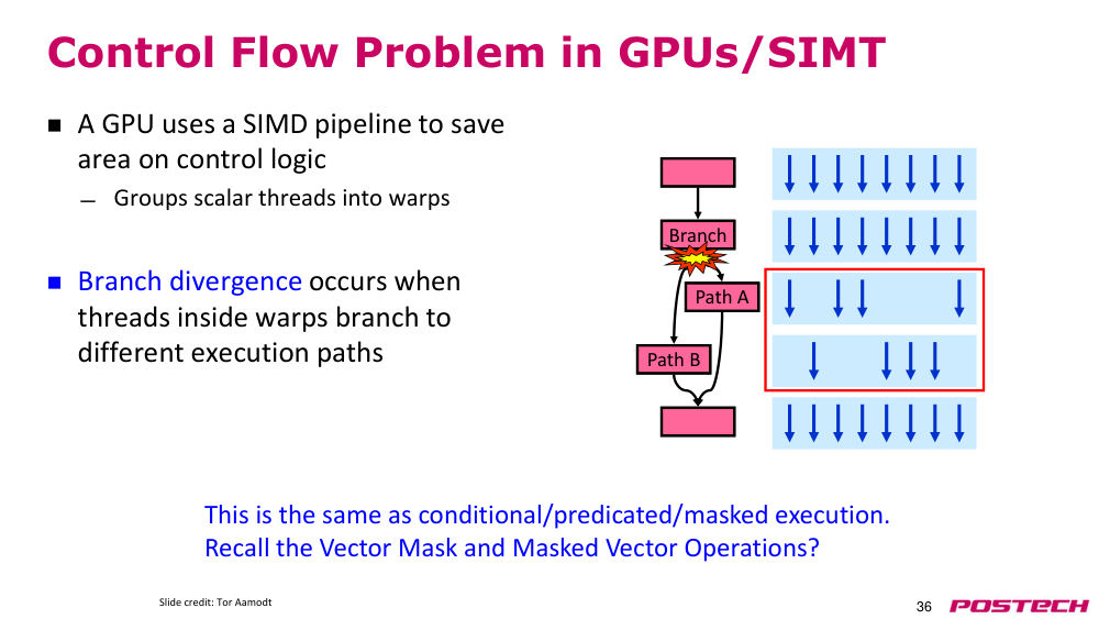
원인warp(32 thread)는 한 instruction 을 함께 실행. branch 로 thread 절반씩 다른 basic block 으로 가면 warp 가 둘로 나뉘어 각 16 thread 만 active.
해결나머지 lane 은 idle → throughput 저하. 해결 실마리: 동시에 도는 다른 warp 중 반대쪽 lane 만 active 인 warp 와 합치기.
- control flow irregularity = control/branch divergence
- basic block G 처럼 경로가 다시 만나면 하나의 warp 로 재결합 가능
- 슬라이드: divergence 는 predicated/masked execution 과 같음
2.3.r.1Wikipedia: Single instruction, multiple threads ↗ · SIMT 의 branch divergence 와 predicate masking
2.415:56–19:32dynamic warp formation(동적 워프 형성)
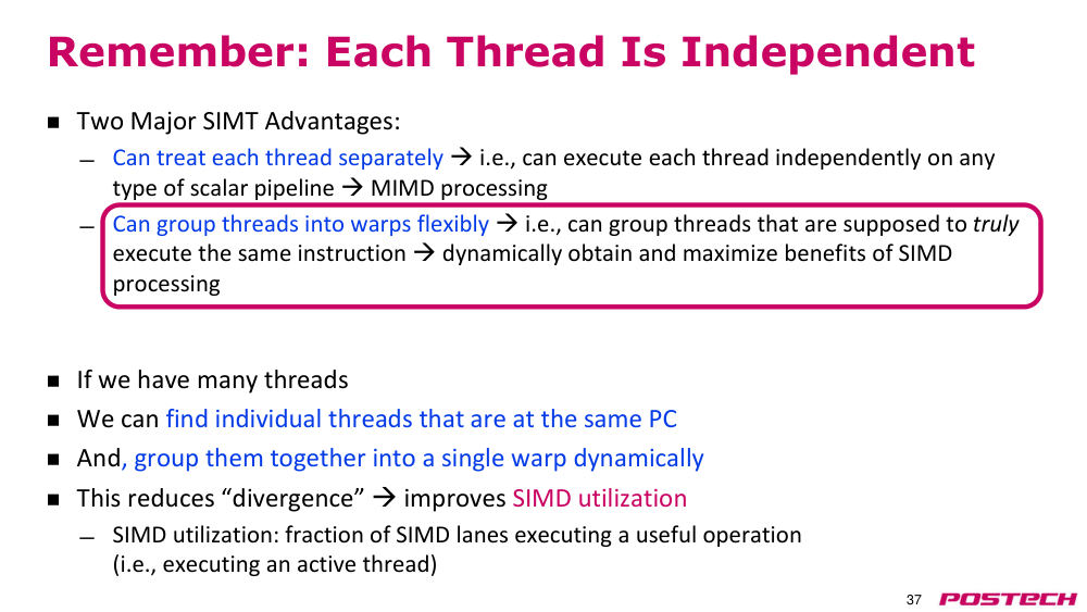
상황·문제SIMT 의 두 장점 중 '유연한 warp 구성' 을 divergence 해결에 활용.
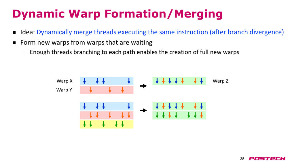
원인같은 PC 에 있는 thread 들을 찾으면 서로 다른 warp 의 부분 active thread 를 한 warp 로 묶을 수 있음.
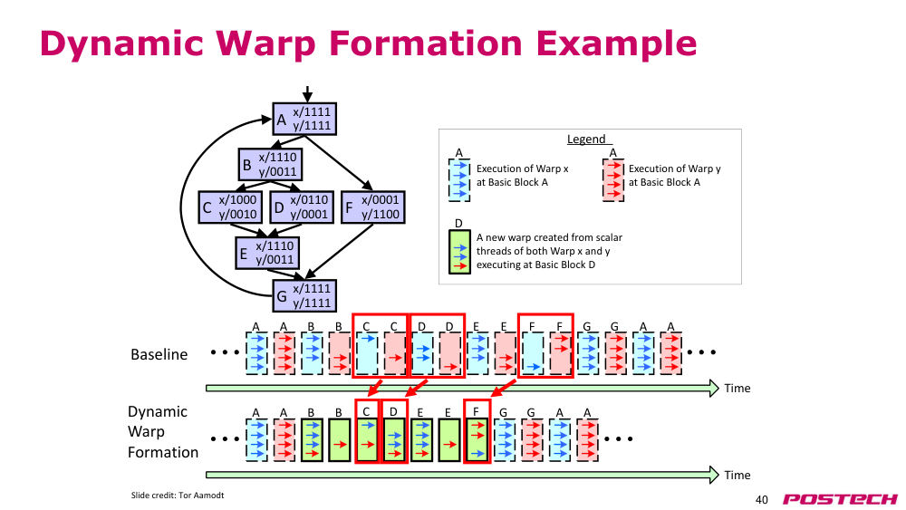
해결Fung et al.(MICRO 2007) dynamic warp formation: 2 cycle 걸릴 두 warp 를 1 cycle 에 실행. 같은 lane 이 겹치면 세 번째 warp 를 끌어와 3 warp → 2 warp.
- divergence 감소 → SIMD utilization 향상
- 겹치는 lane 이 있으면 그대로는 합칠 수 없음
- p40 애니메이션: baseline 대비 C·D·F 구간이 합쳐짐
2.4.r.1Wikipedia: Single instruction, multiple threads ↗ · SIMT 의 branch divergence 와 predicate masking
2.519:32–20:31출석 확인 (행정)
상황·문제GPGPU 마무리(p41 질문·공지 화면) 후 출석 확인, 새 슬라이드 파일(Lecture 22) 열기.
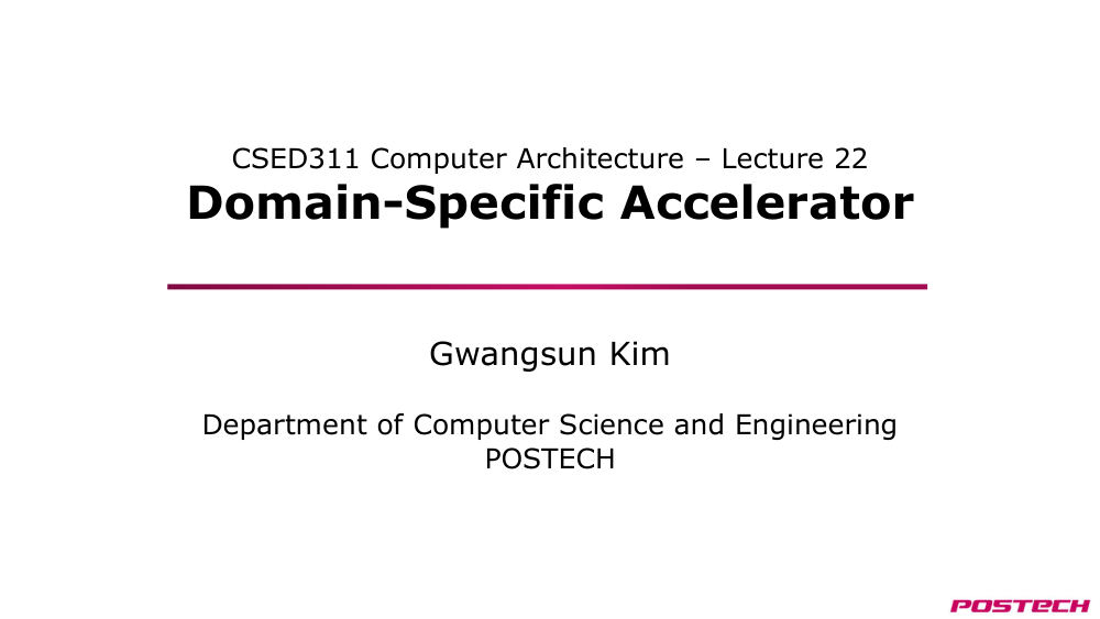
2.620:31–29:05왜 hardware acceleration 인가
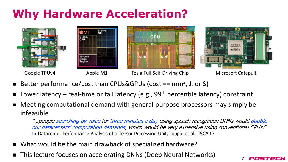
상황·문제특정 application 에 맞게 hardware 를 specialize 하는 domain-specific accelerator. Google TPU, Apple M1 neural engine, Tesla FSD chip, Microsoft FPGA.
원인CPU·GPU 대비 performance/cost(면적·에너지·돈), 낮은 latency 요구, 그리고 Google 의 경우 하루 3분 음성 검색만으로 datacenter 연산 수요가 2배가 될 상황.
해결대신 general-purpose 능력(flexibility)을 잃음. Microsoft 는 flexibility 를 위해 ASIC 대신 재구성 가능한 FPGA 선택. 이번 강의는 DNN 가속에 집중.
- 칩 개발비가 크므로 대규모(예: 100,000 CPU → 1,000 accelerator)여야 이득
- ASIC 은 제작 후 변경 불가, FPGA 는 reconfigure 가능
- TPU 동기: Jouppi et al., ISCA'17 인용문
2.6.r.1Jouppi et al., In-Datacenter Performance Analysis of a Tensor Processing Unit (ISCA'17, arXiv) ↗ · TPUv1 원 논문: 65,536 8-bit MAC matrix unit, software-managed on-chip memory
2.729:05–35:10perceptron 과 MLP: 결국 matrix multiply
상황·문제딥러닝을 안 배운 학생을 위한 DNN 기초.
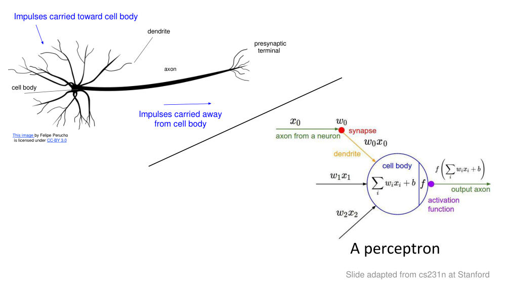
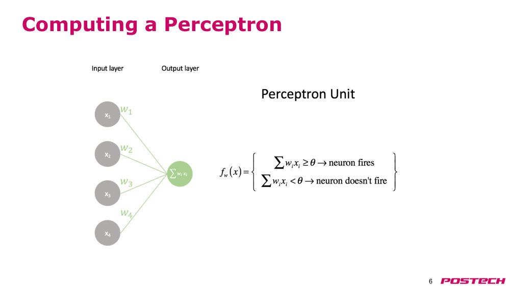
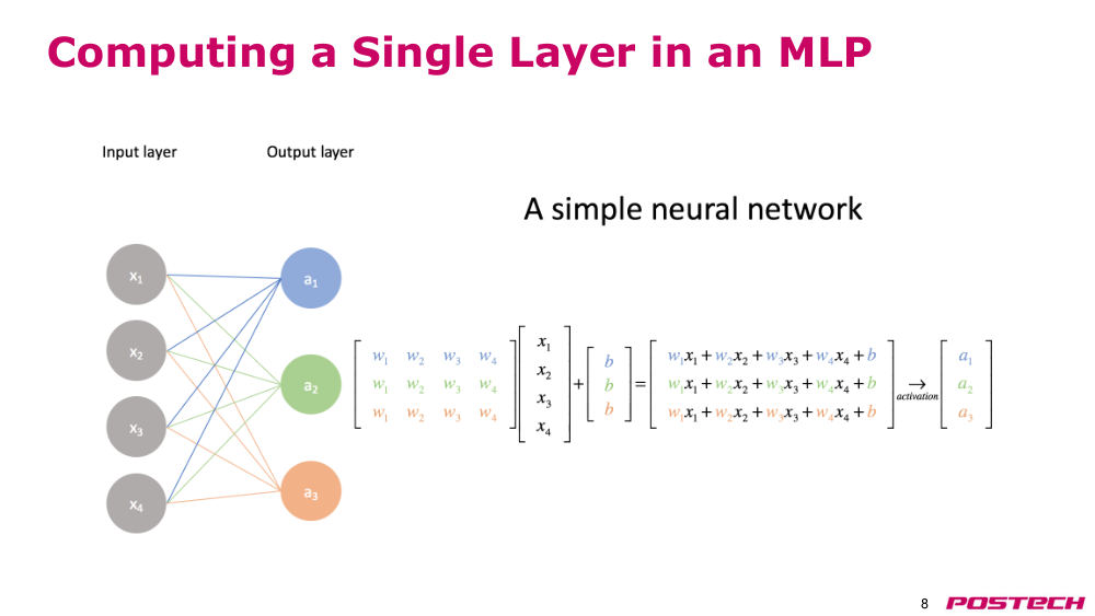
원인perceptron = 입력 x 와 weight 의 dot product + bias → activation function 으로 fire 여부 결정. 여러 perceptron·여러 layer 가 MLP.
해결weight vector 들을 weight matrix 로 묶으면 한 layer 는 matrix×vector + bias, 입력이 여럿이면 matrix×matrix. matrix multiply 가 가속 hardware 의 핵심 building block.
- biological neuron: dendrite 입력 → cell body → terminal 출력
- activation function: sigmoid, tanh, ReLU 등
- MLP 로 classification·regression 수행
2.7.r.1Stanford CS231n: Neural Networks Part 1 ↗ · biological neuron, perceptron, activation function(sigmoid·tanh·ReLU·Leaky ReLU·Maxout)
2.835:13–40:28convolution 연산과 CNN
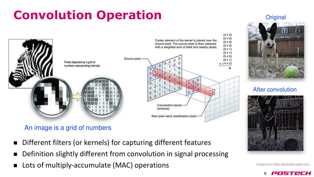
상황·문제computer vision 에서 많이 쓰는 convolution. 이미지는 숫자 grid.
원인3×3 kernel 을 이미지 위에 놓고 9번 multiply-accumulate 해 output 원소 하나, 모든 위치로 sliding 해 feature map 생성. filter 여러 개로 여러 feature.
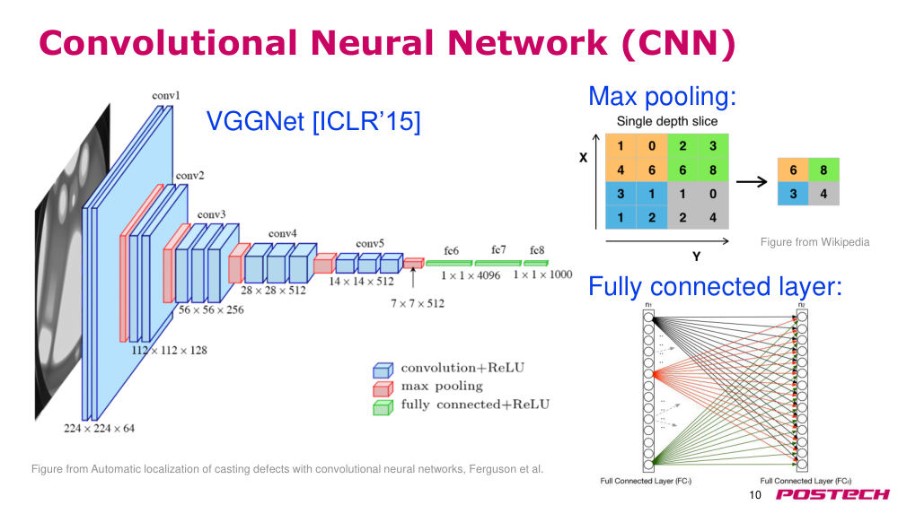
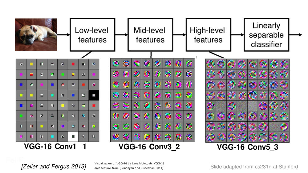
해결conv layer 를 쌓아 고수준 feature 추출(VGGNet), max pooling 으로 feature map 축소, 끝의 fully connected layer(=MLP)가 classifier.
- signal processing 과 달리 kernel 을 flip 하지 않음
- lots of MAC operations
- max pooling = 각 구역의 최댓값 선택
2.8.r.1Stanford CS231n: Convolutional Neural Networks ↗ · conv layer, max pooling, im2col(convolution as matrix multiply), VGGNet
2.940:29–43:20convolution 을 matrix multiply 로 변환
상황·문제convolution 도 matrix multiply hardware 로 처리하고 싶음.
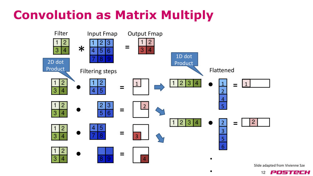
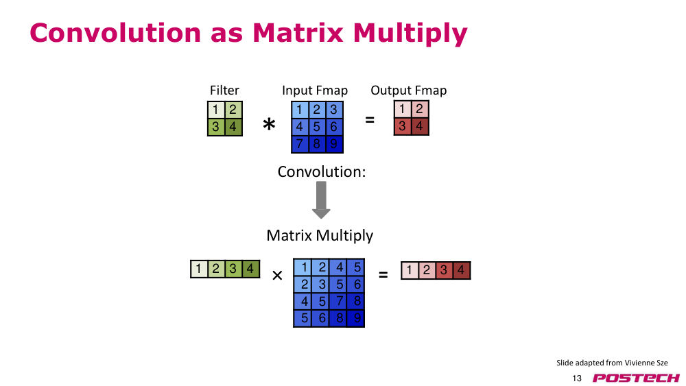
원인각 output 원소는 filter 와 input window 의 2D dot product → flatten 하면 1D dot product.
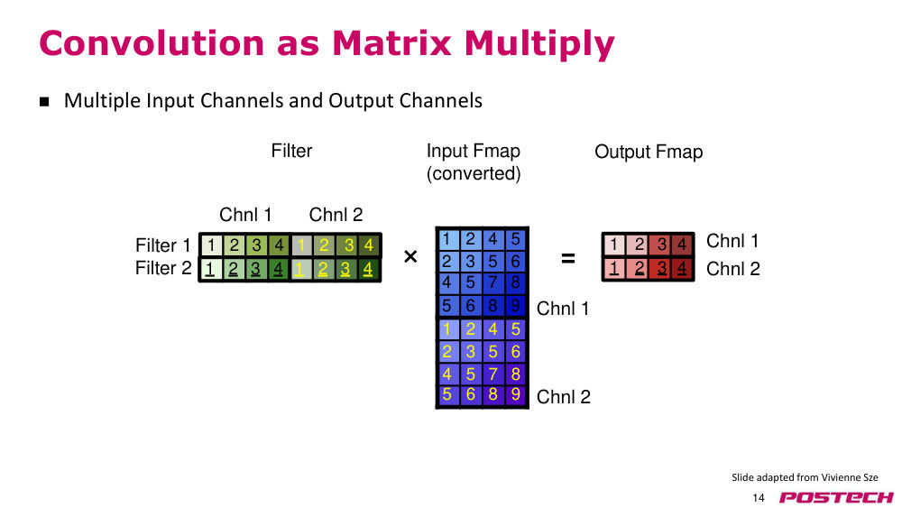
해결window 들을 행렬로 모으면 vector-matrix product. filter 여러 개는 세로로 쌓고, 입력 channel(RGB 등)은 filter 에도 같은 수의 channel 을 가로로 붙임.
- 딥러닝 계산 대부분이 matrix multiply 로 바뀜
- 나머지는 activation·pooling 등
- 그래서 DL hardware 는 matrix multiply 성능이 매우 좋음
2.9.r.1Stanford CS231n: Convolutional Neural Networks ↗ · conv layer, max pooling, im2col(convolution as matrix multiply), VGGNet
2.1043:22–46:07recurrent neural network(RNN)
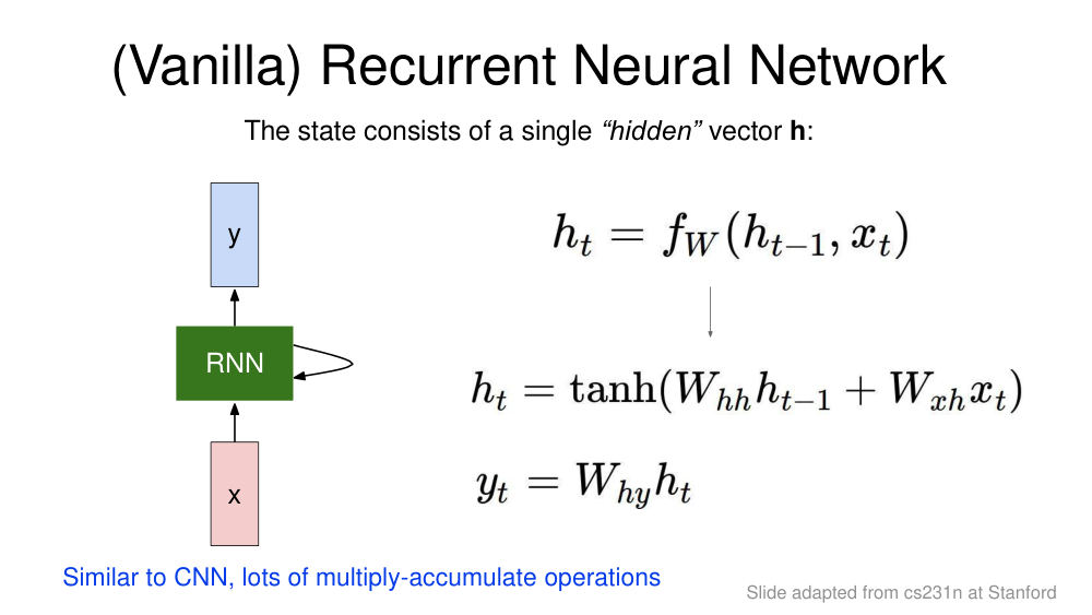
상황·문제앞의 network 는 input 만으로 output 결정. RNN 은 sequential data(예: 영어→한국어 번역)용.
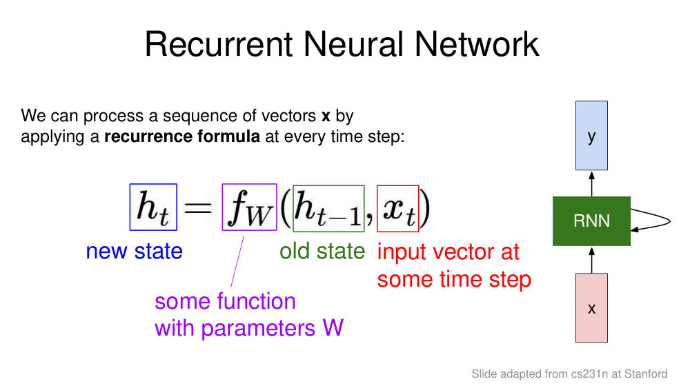
원인output 이 input x_t 와 hidden state h_{t-1} 에 모두 의존.
해결h_t = tanh(W_hh h_{t-1} + W_xh x_t), y_t = W_hy h_t. 결국 weight matrix 곱 + activation, CNN 처럼 MAC 이 많음.
- 단어 하나 = vector 하나, x0, x1, x2… 순서대로 입력
- 문장 끝의 hidden state 로 번역 생성
2.1146:28–52:16training·inference 와 DNN 의 높은 연산 요구
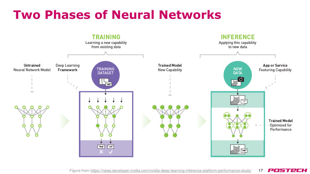
상황·문제weight 값을 처음엔 모름 → training 으로 찾고, 이후 unseen data 에 inference.
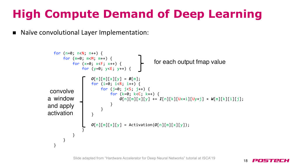
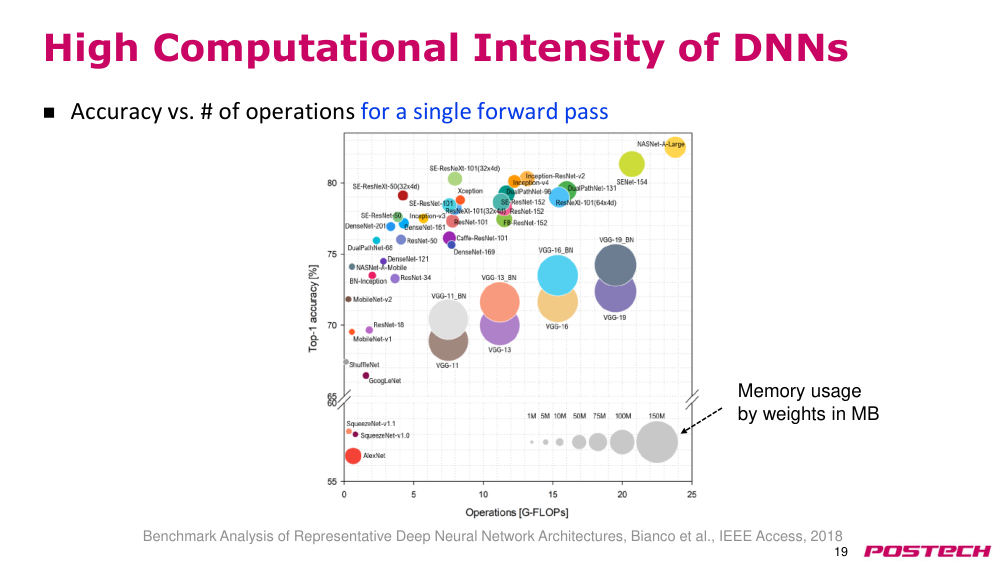
원인naive conv layer 는 7중 for loop, 모델에 따라 layer 수십~수백 개. 정확도가 높을수록 GFLOPs 와 weight memory 가 커지는 추세.
해결이 추세가 고성능 DNN 가속기 개발의 강한 동기.
- training: random init → 예측 결과에 따라 weight 조금씩 수정, 여러 번 반복
- p19 그림: x축 G-FLOPs, y축 accuracy, 원 크기 = weight memory
2.11.r.1NVIDIA Blog: Difference between deep learning training and inference ↗ · training vs inference 두 단계 설명
2.11.r.2Bianco et al., Benchmark Analysis of Representative DNN Architectures (IEEE Access 2018) ↗ · p19 그림 출처: accuracy vs operations vs memory
2.1252:16–58:55systolic array: 개념과 장단점
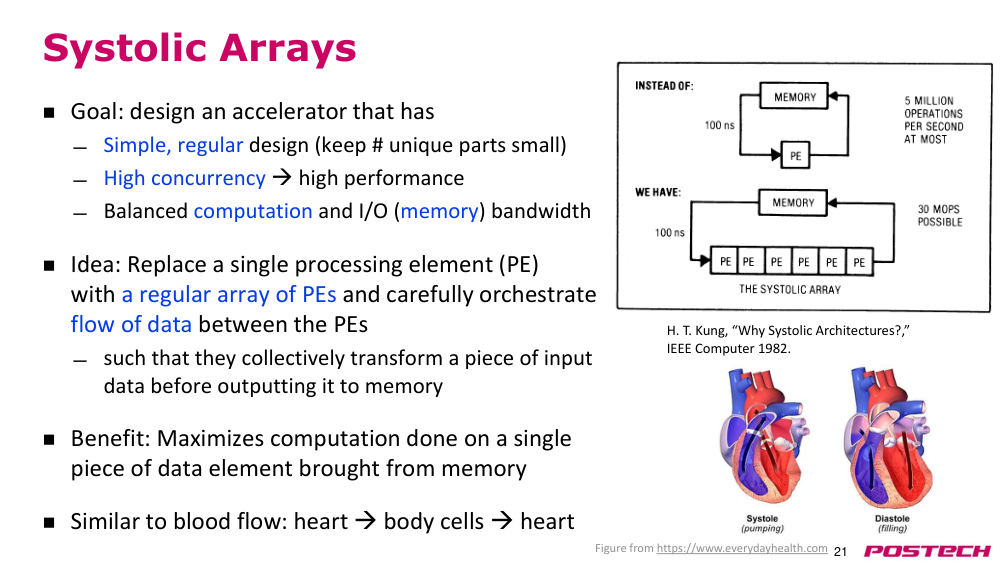
상황·문제가속기 목표: simple·regular design, high concurrency, memory·I/O bandwidth 고려.
원인PE 하나가 연산마다 memory 에 접근하면 memory 가 bottleneck.
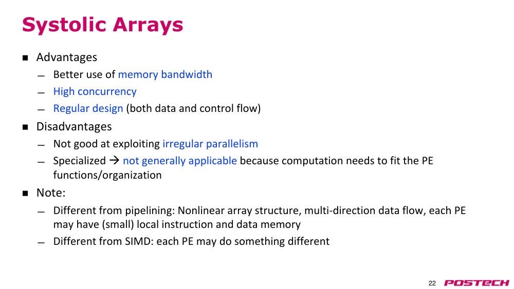
해결PE 배열에서 결과를 다음 PE 로 넘기고 마지막만 memory 로. 예: 5 MOPS → PE 6개로 6배(30 MOPS). 장점 bandwidth 활용·concurrency·regular, 단점 irregular parallelism 에 약하고 범용성 없음.
- 이름은 심장 수축(systole)에서, 데이터가 혈액처럼 순환
- pipelining 과 다름: 비선형 구조·다방향 data flow·PE 별 local memory
- SIMD 와 다름: PE 마다 다른 instruction 가능

2.1358:56–1:02:31systolic array 로 matrix multiply
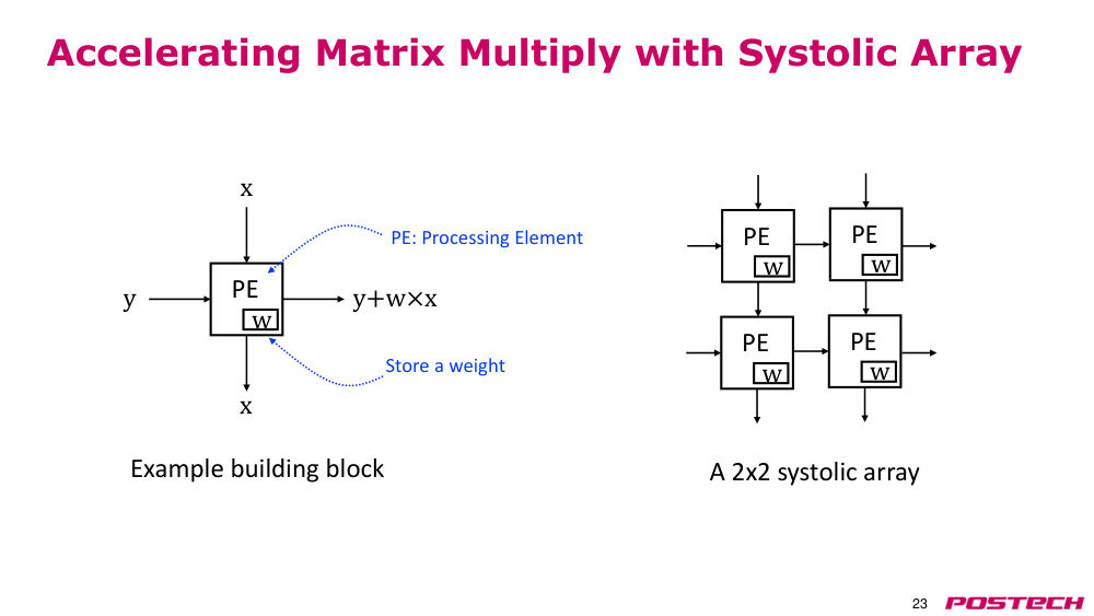
상황·문제PE: weight 저장, x 는 위에서 들어와 아래로 전달, y 는 왼쪽에서 들어와 오른쪽으로 y + w×x 출력.
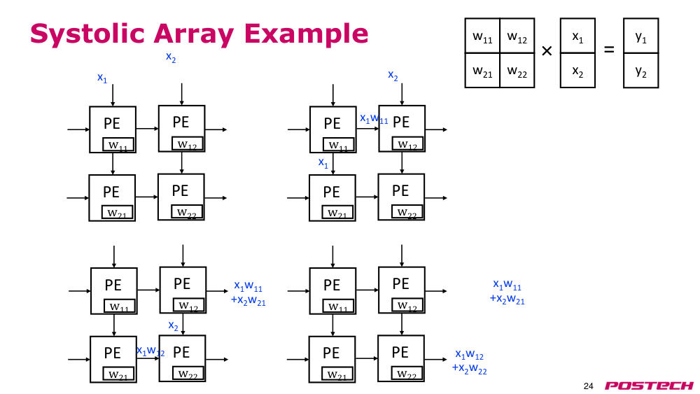
원인2×2 array 에 w11·w12·w21·w22 를 미리 적재하고 x1, x2 를 한 cycle 씩 엇갈려 투입.
해결cycle 마다 x 가 아래로, 부분합이 오른쪽으로 흘러 y1 = x1w11 + x2w21 … 이 나옴. 입력 vector 를 여러 개 묶으면 matrix×matrix.
- time step 1 에는 두 번째 PE 에 입력 없음, 왼쪽 입력은 0
- DL 가속기의 building block
2.141:02:53–1:05:53DSA 설계 지침
상황·문제TPU 를 보기 전에 domain-specific accelerator 지침 정리.
원인범용 cache·데이터 형식·언어로는 domain 의 access pattern·parallelism 을 못 살림.
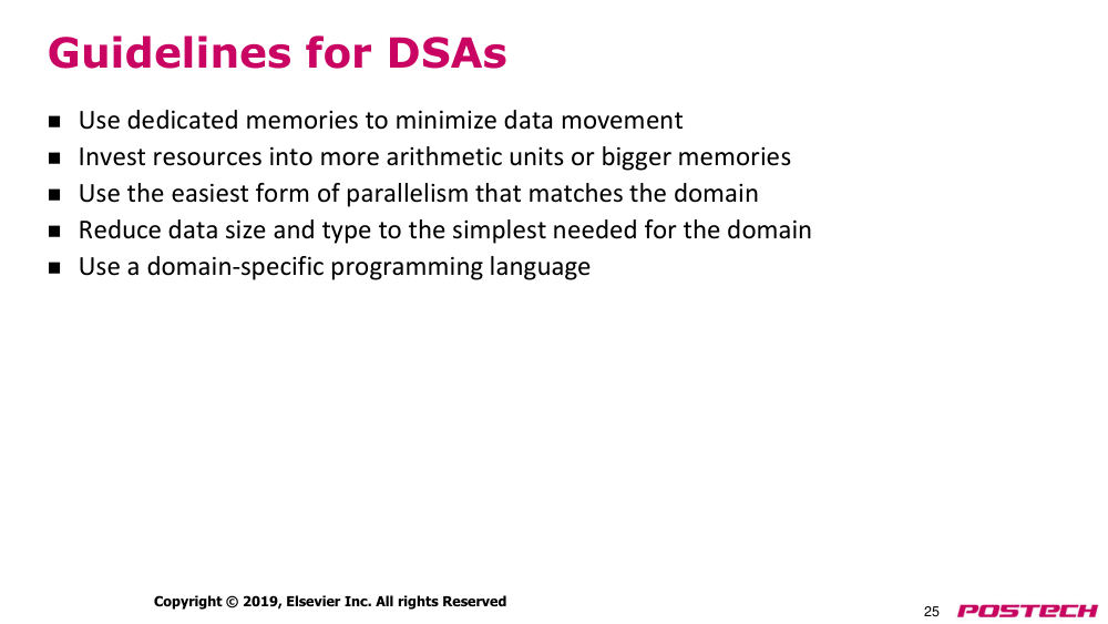
해결dedicated memory(GPU shared memory 처럼 SW 관리), 산술 유닛·큰 on-chip storage·고대역 DRAM 에 투자, domain 에 맞는 가장 쉬운 parallelism, 최소 data type(예: half precision), domain-specific language.
- cache 대신 SW 가 관리하는 special memory
- 7중 loop 로 쓰면 regular pattern 을 자동 추출하기 어려움 → 전용 언어
2.151:05:54–1:12:06Google TPU(v1): 구조와 ISA
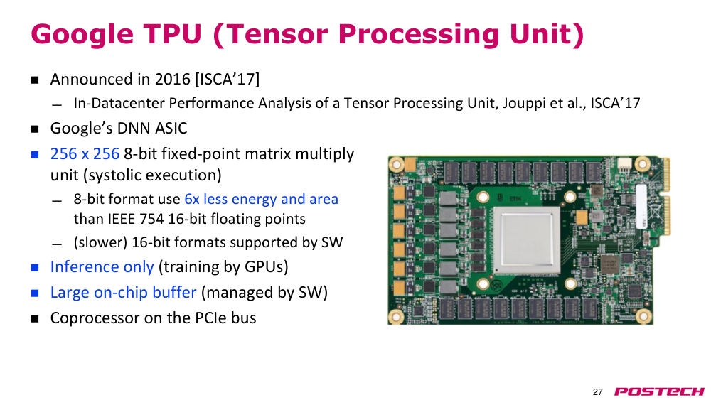
상황·문제2016 발표, ISCA 2017 논문. inference 전용 ASIC, PCIe 로 붙는 coprocessor.
원인256×256 systolic array, 8-bit fixed point(16-bit FP 대비 energy·area 6배 절감, 16-bit 은 SW 로 느리게). training 은 GPU 등 다른 processor.
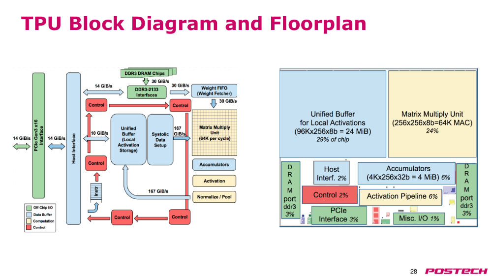
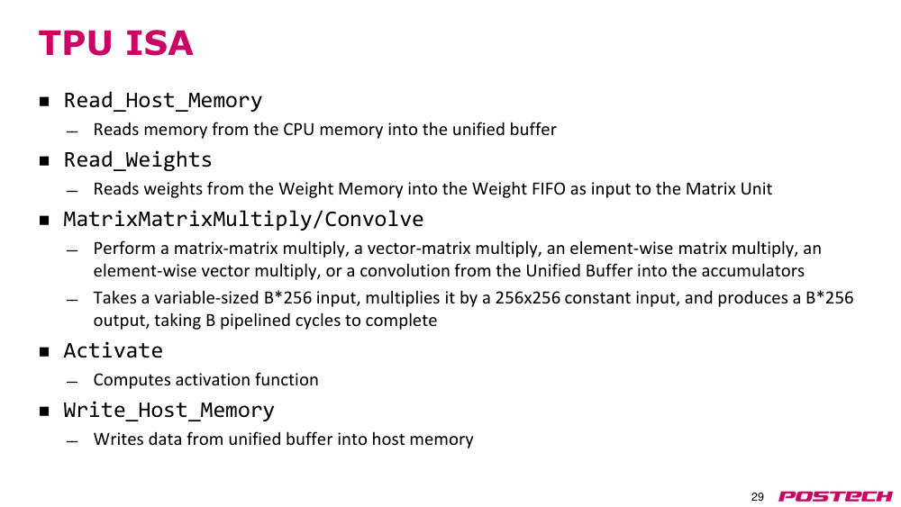
해결weight FIFO·unified buffer → systolic data setup → MMU → accumulator·activation·normalize/pool → unified buffer. CISC 형 ISA: Read_Host_Memory, Read_Weights, MatrixMultiply/Convolve, Activate, Write_Host_Memory.
- floorplan: unified buffer 24 MiB(슬라이드 29% of chip), MMU 24%
- MatrixMultiply 는 가변 크기 입력, 여러 cycle 소요
- 강의는 여기까지, 나머지는 다음 시간
2.15.r.1Jouppi et al., In-Datacenter Performance Analysis of a Tensor Processing Unit (ISCA'17, arXiv) ↗ · TPUv1 원 논문: 65,536 8-bit MAC matrix unit, software-managed on-chip memory
2.15.r.2Google Cloud Blog: An in-depth look at Google's first TPU ↗ · 256x256 systolic MXU, 8-bit quantization, Read_Host_Memory 등 CISC 명령 해설
2.161:12:08–1:14:05Q&A: 왜 TPUv1 은 inference 만?
상황·문제학생 질문: 왜 inference 만 지원했나.
원인교수 추측: training 은 GPU 에서 한 번, inference 는 많은 사용자 요청에 반복 → 더 큰 문제였을 것. training 도 inference 를 포함하므로 공통 부분부터.
해결이후 TPU 세대는 training 도 지원. 진짜 이유는 모른다며 논문 참고를 권함.
- 교수 본인 추측임을 명시
2.16.r.1Jouppi et al., In-Datacenter Performance Analysis of a Tensor Processing Unit (ISCA'17, arXiv) ↗ · TPUv1 원 논문: 65,536 8-bit MAC matrix unit, software-managed on-chip memory
3핵심 개념
3.1thread index(스레드 인덱스)
i = threadIdx.x + blockDim.x * blockIdx.x. 1D grid 에서 각 thread 가 맡을 원소.
3.1.r.1Wikipedia: Thread block (CUDA programming) ↗ · i = blockIdx.x*blockDim.x + threadIdx.x 인덱싱, warp=32 thread
3.2cudaMalloc / cudaMemcpy
GPU memory 할당과 host↔device 복사. CPU·GPU memory 는 분리.
3.3control divergence(제어 분기)
warp 내 thread 가 branch 로 다른 경로 → 일부 lane 만 active, utilization 저하.
3.3.r.1Wikipedia: Single instruction, multiple threads ↗ · SIMT 의 branch divergence 와 predicate masking
3.4dynamic warp formation(동적 워프 형성)
같은 PC 의 thread 를 여러 warp 에서 모아 새 warp 구성. Fung et al., MICRO 2007.
3.5domain-specific accelerator(DSA, 도메인 특화 가속기)
특정 application 용으로 specialize 한 hardware. performance/cost 이득, flexibility 손실.
3.6ASIC vs FPGA
ASIC 은 제작 후 변경 불가, FPGA 는 reconfigure 가능. Microsoft 는 flexibility 위해 FPGA.
3.7perceptron(퍼셉트론)
입력·weight dot product + bias → activation function 으로 fire 결정.
3.7.r.1Stanford CS231n: Neural Networks Part 1 ↗ · biological neuron, perceptron, activation function(sigmoid·tanh·ReLU·Leaky ReLU·Maxout)
3.8convolution(컨볼루션)
kernel 을 sliding 하며 MAC 으로 feature map 생성. DL 에선 kernel flip 없음.
3.8.r.1Stanford CS231n: Convolutional Neural Networks ↗ · conv layer, max pooling, im2col(convolution as matrix multiply), VGGNet
3.9max pooling(맥스 풀링)
구역별 최댓값으로 feature map 크기 축소.
3.9.r.1Stanford CS231n: Convolutional Neural Networks ↗ · conv layer, max pooling, im2col(convolution as matrix multiply), VGGNet
3.10RNN(순환 신경망)
h_t 가 h_{t-1} 과 x_t 에 의존. sequential data 처리.
3.11training / inference(학습 / 추론)
training 으로 weight 를 찾고, inference 로 새 입력을 예측.
3.11.r.1NVIDIA Blog: Difference between deep learning training and inference ↗ · training vs inference 두 단계 설명
3.12systolic array(시스톨릭 어레이)
PE 배열에서 데이터가 흐르며 memory 접근 없이 여러 단계 처리. regular·high concurrency.
3.14TPU(Tensor Processing Unit)
Google 의 DNN inference ASIC. 256×256 8-bit systolic MMU, PCIe coprocessor.
3.14.r.1Jouppi et al., In-Datacenter Performance Analysis of a Tensor Processing Unit (ISCA'17, arXiv) ↗ · TPUv1 원 논문: 65,536 8-bit MAC matrix unit, software-managed on-chip memory
3.14.r.2Google Cloud Blog: An in-depth look at Google's first TPU ↗ · 256x256 systolic MXU, 8-bit quantization, Read_Host_Memory 등 CISC 명령 해설
3.15unified buffer(통합 버퍼)
TPU 의 24 MiB SW 관리 on-chip storage. 입력·출력 activation 보관.
3.15.r.1Google Cloud Blog: An in-depth look at Google's first TPU ↗ · 256x256 systolic MXU, 8-bit quantization, Read_Host_Memory 등 CISC 명령 해설
4스스로 확인
4.1N=1024, block 당 256 thread 일 때 blockIdx.x=2, threadIdx.x=10 thread 의 index 는?
답
256×2+10 = 522.
4.2vector_add 실행 전 host 가 해야 할 두 가지 CUDA 호출은?
답
cudaMalloc 으로 d_A·d_B·d_C 할당, cudaMemcpy(HostToDevice) 로 A·B 복사.
4.3branch divergence 가 GPU throughput 을 떨어뜨리는 이유는?
답
warp 는 한 instruction 만 실행하므로 경로별로 나눠 실행, 그동안 나머지 lane 이 idle.
4.4dynamic warp formation 으로 두 부분 warp 를 합칠 수 없는 경우는?
답
같은 lane 의 thread 가 두 warp 모두에서 active 일 때. 다른 warp 를 더 찾아 재배치해야 함.
4.5specialized hardware 의 주된 단점과 Microsoft 의 선택은?
답
general-purpose 계산 능력(flexibility) 손실. 그래서 ASIC 대신 FPGA.
4.6convolution 을 matrix multiply 로 바꾸는 핵심은?
답
각 window 의 2D dot product 를 flatten 해 1D 로, window 들을 행렬로 모음.
4.7PE 6개 systolic array 가 memory-bound baseline 5 MOPS 대비 얻는 성능은?
답
memory 를 한 번만 거치므로 6배, 30 MOPS.
4.8TPUv1 이 8-bit fixed point 를 쓴 이유는?
답
초기 용도에 충분했고 16-bit FP 대비 energy·area 6배 절감.
5참고 자료
5.1Jouppi et al., In-Datacenter Performance Analysis of a Tensor Processing Unit (ISCA'17, arXiv) ↗ · TPUv1 원 논문: 65,536 8-bit MAC matrix unit, software-managed on-chip memory
5.2Google Cloud Blog: An in-depth look at Google's first TPU ↗ · 256x256 systolic MXU, 8-bit quantization, Read_Host_Memory 등 CISC 명령 해설
5.4Stanford CS231n: Neural Networks Part 1 ↗ · biological neuron, perceptron, activation function(sigmoid·tanh·ReLU·Leaky ReLU·Maxout)
5.5Stanford CS231n: Convolutional Neural Networks ↗ · conv layer, max pooling, im2col(convolution as matrix multiply), VGGNet
5.6Wikipedia: Thread block (CUDA programming) ↗ · i = blockIdx.x*blockDim.x + threadIdx.x 인덱싱, warp=32 thread